The Easy Guide To The GETPIVOTDATA Function In Excel

Are you looking for a way to quickly analyze data in Microsoft Excel?

The GETPIVOTDATA function is an incredibly powerful tool that can help you easily extract and manipulate data from pivot tables. This function lets you quickly get the exact information you need without manually searching through your spreadsheet. Plus, it’s easy to use!

Imagine accessing all of the data stored in your pivot table with just one simple formula. You won’t have to spend time searching for the right cell or scrolling through rows of numbers – instead, you’ll be able to instantly get the answers you need.

Read on and learn how to use the GETPIVOTDATA function in Microsoft Excel today!

What Is An Excel Pivot Table?

Before you can use the GETPIVOTDATA function, it’s essential to understand what a pivot table is. A pivot table is a powerful tool that allows you to quickly organize, summarize, and analyze large amounts of data.

A pivot table contains rows and columns of information from your original data set. You can then manipulate the pivot table layout to display various data summaries, such as sums, averages, and counts.

For example, let’s say you have a spreadsheet containing sales data for your company. You can use a pivot table to quickly determine which product was the best seller in each region or which month had the highest average sales. You could also use the pivot table to calculate total sales by region or find out which products had the largest increase in sales from one period to the next.

What Is The GETPIVOTDATA Function In Excel?

The GETPIVOTDATA function is a powerful tool in Excel that enables you to extract data from a specified pivot table. This function helps you quickly get the exact information you need without manually searching through your spreadsheet or table.

What are the advantages of GETPIVOTDATA?

Querying pivot table data with GETPIVOTDATA has several advantages. It’s much more efficient than writing a traditional formula for extracting values from a pivot table. It also makes formulas easier to read and understand since you don’t have to look up the internal names of each field when writing the formula.

Additionally, querying with GETPIVOTDATA reduces the risk of errors since it can’t return incorrect values. When entered incorrectly, traditional formulas are prone to returning inaccurate results. Lastly, you can use GETPIVOTDATA to query multiple pivot tables at once and quickly get consolidated data from all tables.

What is the difference between GETPIVOTDATA and VLOOKUP in Excel?

Querying a pivot table with GETPIVOTDATA significantly differs from querying a table with VLOOKUP. VLOOKUP allows you to search for information in a specific column of one or more tables and then returns the corresponding value from any other column within that table.

On the other hand, GETPIVOTDATA queries a pivot table structure and returns the correct data from any combination of rows, columns, or values in the table. It is not limited to returning only values from one specific column. GETPIVOTDATA also has the ability to reference a hidden pivot table field, which can be helpful when you need to query information that isn’t visible on the screen.

What is the difference between GETPIVOTDATA and SUMIFS in Excel?

GETPIVOTDATA and SUMIFS are both formulas in Microsoft Excel for finding data within a given set of criteria. The main difference between them is the type of data they search through. GETPIVOTDATA can retrieve data stored in pivot tables, while SUMIFS searches through a table or range of cells.

The GETPIVOTDATA Formula Syntax

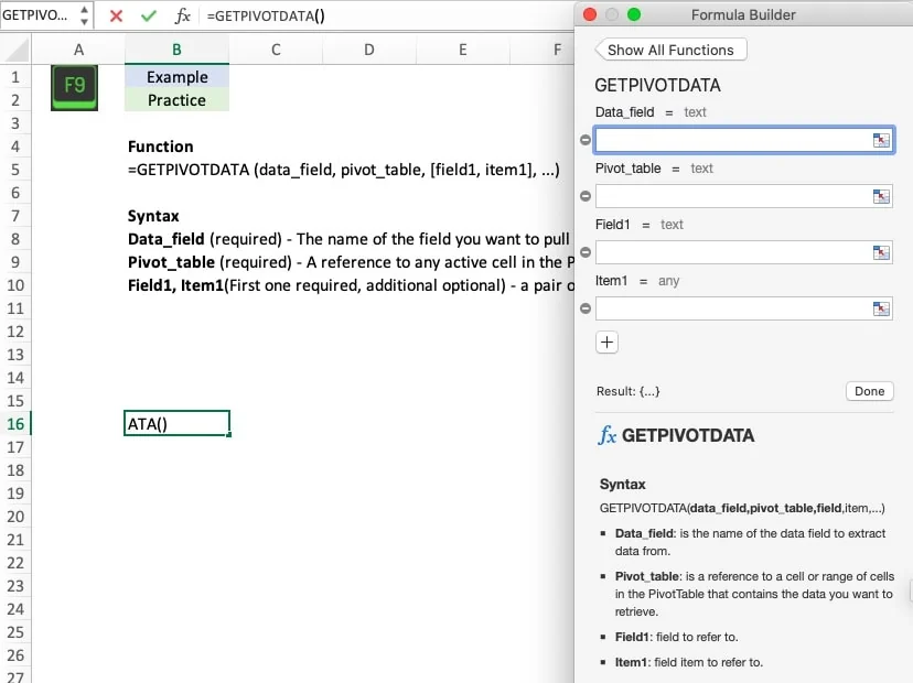
Here is the GETPIVOTDATA function syntax:

=GETPIVOTDATA(data_field, pivot_table, [field1, item1], …)

• Data_field (required) – The name of the field you want to pull from the Pivot Table
• Pivot_table (required) – A cell reference in the Table or the name of the Table that you want to pull pivot data from
• Field1, Item1(First one required, additional optional) – a pair of fields and items that you want to pull

Where Is The Excel GETPIVOTDATA Function located?

Option 1:

You can find the GETPIVOTDATA function in the Formulas tab of Excel under Lookup & Reference.

Option 2:

You can use Formula Builder to walk you through the formula step by step.

Option 3:

You can manually type the formula into any cell.

How To Use The GETPIVOTDATA Function

Excel Workbook

Example – Analyze Store Performance

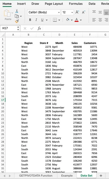
Let’s walk through an example of using GETPIVOTDATA to analyze the performance of a chain of retail stores spread across the country. We can use pivot tables to quickly manipulate a large data set. Our data set has sales and customer data by month for various stores across four regions.

Now that we have the data, we will generate a pivot table using the data set. Let’s put regions across the columns, months down the rows, and sum sales.

Now let’s work with the GETPIVOTDATA function. First, we will pull total sales for the east region. The formula is =GETPIVOTDATA(“Sales”, $F$5, “Region”, C7). We want to pull Sales as the data field. $F$5 is the top left corner of the pivot table we want to pull from, and “Region” / “East” (linked to C7) is the data pair.

For the second example, we keep region and also add in “Month” as a second data pair.

Your turn: Use the workbook and GETPIVOTDATA to follow the examples in blue and finish the practice formulas highlighted in green. Hint, you will need to repivot the table.

Real-Life Case Studies

Case Study 1: Retail Sales Analysis Made Easy with GETPIVOTDATA

The Scenario:

Meet Sarah, the sales manager for Trendy Threads, a fast-growing retail company that sells everything from chic apparel to accessories. Sarah’s job is to keep tabs on sales performance across multiple regions and product categories. Her team creates robust pivot tables in Excel to summarize the mountain of daily transactions. The problem? Every time Sarah needed specific numbers – say, how many units of their best-selling denim jackets sold in the West region last month – she’d resort to manually filtering the data or eyeballing rows in the pivot table. Not efficient. Not scalable.

Enter GETPIVOTDATA:

With GETPIVOTDATA, Sarah found a way to extract exactly the numbers she needed – no filters, no guesswork, no manual digging. She learned the function could directly reference the pivot table in her report, pulling out customized insights with laser accuracy.

The Solution in Action:

One Monday morning, Sarah needed to analyze July’s sales data to prep for a team meeting. Using a pivot table, she organized sales by region and product category. Then she created a dashboard for her team, linking sales metrics from the pivot table to specific cells using GETPIVOTDATA. Here’s how she did it for those denim jackets in the West region:

=GETPIVOTDATA("Sales", $A$3, "Region", "West", "Category", "Denim Jackets")

• “Sales”: The field she wanted to extract.
• $A$3: A cell within the pivot table, allowing Excel to recognize the data source.
• “Region”, “West”, “Category”, “Denim Jackets”: The criteria to zero in on the exact metric.

The Results:

Within seconds, Sarah had her number. Sales for denim jackets in the West totaled $12,300. Even better? When the pivot table updated to reflect newly added data, the GETPIVOTDATA function updated automatically, ensuring her dashboard was always accurate.

Sarah took GETPIVOTDATA one step further by integrating it into sales targets. When her CEO asked for a report on whether each region hit their product-specific sales goals, Sarah effortlessly pulled together a real-time report. The dashboards were so on point, her coworkers joked she must have had insider intel.

Case Study 2: Quarterly Financial Reporting Without the Chaos

The Scenario:

Raj, a financial analyst at GreenStreet Capital, dreaded quarterly reporting. His team used pivot tables – naturally – to summarize their firm’s financial data. But breaking down specific figures for revenue, expenses, and profit by department always felt like a house of cards. One accidental change in the pivot table structure could break half his Excel formulas. And updating the report every quarter? Painful.

Raj needed a solution that would not only speed up his process but ensure that his numbers were rock solid every single time. That’s when he uncovered the beauty of GETPIVOTDATA.

The Solution in Action:

Raj used a pivot table to summarize key financial metrics for the quarter. Then, to simplify the report-building process, he used GETPIVOTDATA to extract and display specific numbers for his company’s leadership team. For example, when his CFO asked for Q3 revenue for the Technology division, Raj used this formula:

=GETPIVOTDATA("Revenue", $B$4, "Quarter", "Q3", "Department", "Technology")

• “Revenue” captured revenue figures from the pivot table.
• $B$4 anchored the reference to the original pivot table.
• “Quarter”, “Q3”, “Department”, “Technology”: Pinpointed the exact metric without worrying about changes to the layout.

For finalizing the income statement, Raj also pulled other metrics like operating expenses and total profit using similar formulas.

The Results:

By using GETPIVOTDATA, Raj’s report game transformed. No matter how the pivot table layout changed – whether someone moved rows, columns, or even fiddled with the filters – his formulas stayed intact. What used to take him entire afternoons now took just a few minutes.

When the CFO threw a curveball, asking for a quick snapshot of total revenue across all departments, GETPIVOTDATA didn’t flinch. Raj adjusted his criteria, and the numbers popped up instantly. His quarterly reporting transitioned from chaotic to clockwork. And as a nice bonus, when external auditors reviewed their financials, Raj could confidently prove every single figure was accurate and directly linked to raw data.

Tips and Tricks

Better Together

GETPIVOTDATA works in tandem with any other function that can use a value. It pairs especially well with SUM, AVERAGE, MIN, and MAX Functions.

Watch Your Spelling

GETPIVOTDATA will return a #REF error if you misspell any of your entries or if it can’t find the field you are referencing. You will receive the same error if any of the cell references are entered incorrectly.

I’m Late For A Very Important Date

When working with the pivot table’s date format (or time format), use Excel’s “Date and Time” functions in the formula to ensure everything pulls correctly and in the same date format. Examples include DATEVALUE Function and DATE Function.

Turning GETPIVOTDATA On Or Off

Starting in Excel 2007, you can turn off automatic formula writing for GETPIVOTDATA functions using a command in the Excel Ribbon.

• First, select any cell in a pivot table.
• Then, go to the Ribbon and click the PivotTable Analyze tab.
• From there, click the arrow on the PivotTable command and then click the drop-down arrow for Options.
• Finally, click the Generate GETPIVOTDATA command, to turn the feature off or on.