
Pie Charts in Excel
Pie charts look complex but are super easy to create in Excel. Let’s walk through what a pie chart is, how to insert it, and an example to put it into practice.
What is a Pie Chart?
A pie chart is a circular graphic divided into slices. Each slice represents an individual category and its percentage of a whole.
Let’s think about this in a business context. Let’s say that you want to show sales product mix. This is perfect for a pie chart! Each product will be one slice of the total product sales. Or, let’s say that you want to look at sales by region. Each slice can be a region adding up to total sales.
How to Insert a Chart
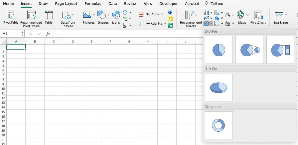
Charts can be found on the Insert tab of the ribbon. Once you are on the Insert tab, select the pie charts dropdown (icon of a pie). There are subset versions of the pie chart to show extra detail, along with a 3D pie chart and a doughnut chart.
You will need to apply the chart to an existing data set. We will walk through this in more detail in the example. I’d recommend sticking to 2D charts versus 3D until you feel comfortable.
Example – Sales Volume by Product or Region:
Step 1: Layout data set
First, you will need the data set to include in the chart. For our example, we will look at sales volume by product by region for a full year period.

Step 2: Select Range and Insert Chart
To insert a chart, you first need to highlight the data range. Make sure to pull in only the headers for product type or region as a pie chart can only work with one set of headers. Excel will automatically pull in the headers for you.
Once you have highlighted the range, insert a standard pie chart following the instructions above.

Step 3: Format the Chart
Excel will create the chart with default formatting, doing its best to scale, label, and make the chart readable. This was what Excel’s first crack at it looked like:

That said, you will often want to tweak the formatting for personal preference or company brand standards.
To adjust the formatting, you can click on any part of the chart that you want to edit. You can click on the gridlines to remove them, the axis to adjust the scale, the bars to change the color scheme, really anything you want. Also note that when you select a chart, two additional tabs are added to the ribbon. The tabs are “Chart Design” and “Format” and will help you with changes.
We will make the following changes to the chart:
- Click on the title and hit delete
- Click on the product types and bold them
- Go to chart design, change colors, and select the blue gray pattern
- Right click on the chart, add data labels, format as a percentage. Click the data labels, bold them, and make the font white.
Here is the end result of our changes that looks a lot more executive presentation ready:

Learn More About Excel
To learn more about Excel, you need training and practice. To find the best options for training, check out our post on the Best Excel Courses and start your learning journey today.
Have any questions on pie charts in Excel? Are there other topics you would like us to cover? Leave a comment below and let us know! Make sure to subscribe to our Newsletter to receive exclusive financial news right to your inbox.