
How to Use the HYPERLINK Function in Excel
Do you want to create a hyperlink in Excel that your users can click on to open another file or page? The HYPERLINK function makes it easy to do just that! In this blog post, we will discuss how to use the HYPERLINK function in Excel and show you some examples of how it can be used. We will also show you how to make your links look pretty and user-friendly. So, let’s get started!
What Does The HYPERLINK Function Do?
The HYPERLINK function returns a hyperlink from a given destination and link text. You can use HYPERLINK to create a clickable hyperlink with a formula. The HYPERLINK function can build links to workbook locations, pages on the internet, or files on network servers. When a user clicks a cell that contains the HYPERLINK function, Excel will open the file or page specified by link_location.
Where To Find It?
Option 1:
You can find the HYPERLINK function in the Formulas tab of Excel under Lookup & Reference
Option 2:
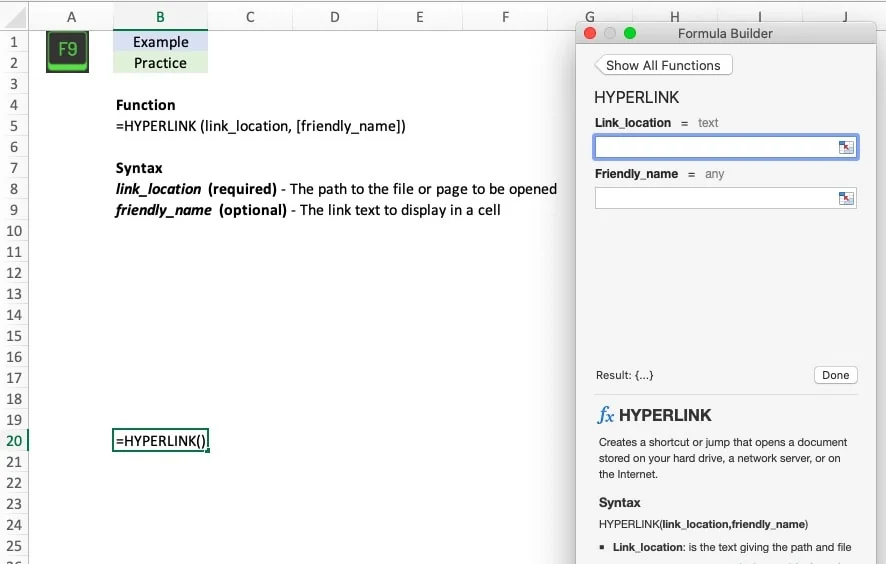
You can use Formula Builder to walk you through the formula step by step.
Option 3:
You can manually type the formula into any cell.
The Formula
=HYPERLINK (link_location, [friendly_name])
- link_location (required) – The path to the file or page to be opened
- friendly_name (optional) – The link text to display in a cell
Let’s Take a Look at Some Real-World Examples
Excel Workbook
Example
In the first example pair, we will create hyperlinks within the workbook. Let’s create a hyperlink to the syntax for the function. Remember to encase all of the arguments in quotation marks. The formula is =HYPERLINK(“#HYPERLINK Function!A1”, “Function Syntax”). This creates a direct link to the other tab in the workbook with a friendly_name of Function Syntax.
Next, we will create a hyperlink to a website. We will point to Seeking Alpha, a great reference for stock market insights. The formula is =HYPERLINK(“www.seekingalpha.com”, “Stock Data”). This creates a link to the home page of Seeking Alpha with a friendly_name of Stock Data.

Your turn: Use the workbook and HYPERLINK to follow the examples in blue and finish the practice formulas highlighted in green.
Tips and Tricks
I Can’t Click The Cell
The default when you try to click a HYPERLINK cell is to follow the link. You will need to arrow over to the cell to modify the formula.
Links To Parts Of Your Spreadsheet
You can create links to different parts of your workbook by placing a # in front of a cell reference, a sheet reference, or a named range.
Receiving An Error
The most common error occurs when the link path cannot be followed, check to make sure that you entered the link exactly as it appears. Also, make sure that the friendly_name is in quotations.
Let’s Recap
In today’s blog post, we discussed how to use the HYPERLINK function in Excel. We showed you how to create links to different parts of your workbook and explained some of the most common errors that can occur. We hope you found this information helpful!
Have any questions? Are there other topics you would like us to cover? Leave a comment below and let us know! Make sure to subscribe to our Newsletter to receive exclusive financial news right to your inbox.