
Master the Magic of SUM Functions in Excel
Ever find yourself knee-deep in receipts at the end of a long, busy day, wishing there was a magic wand that could instantly add up all your sales? Well, what if I told you that Excel’s SUM function is that magic wand, ready to turn your number-crunching nightmares into a dream come true?
This article will focus on one of Excel’s most powerful weapons – the SUM function. We’ll start with the basics, gradually moving towards its variations like SUMIF, SUMIFS, and SUMPRODUCT. Don’t worry if these terms sound intimidating right now. By the end of this guide, I promise you’ll be wielding these functions like a pro, ready to take charge of your business finances.
So, buckle up and prepare for an exciting journey into Excel and business finance. Let’s make that spreadsheet shine!
Quick Overview
Using the Excel Sum Function is straightforward. Just type =SUM( in a cell, then select the range of cells you want to add together. Close the parentheses and hit Enter. For example, =SUM(A1:A10) will add all the values in cells A1 through A10.
Understanding The Excel SUM Function
Let’s dive right in and get to know our star of the day a little better – the SUM function. Imagine you’re at a party, and you’ve been tasked with collecting all the empty soda cans. You could go around counting each can individually, but that would take forever! Instead, you decide to group them into piles of ten for easier counting. This is essentially what the SUM formula does. It adds up a bunch of numbers (or soda cans, if you will) so you don’t have to do it manually.
In Excel language, SUM is a function that adds up all the numbers in a specific range of cells. So, instead of manually adding numbers like 10 + 20 + 30, you just tell Excel to SUM them up, and voila! You’ve got your total.
Now, you might be thinking, “Sure, that sounds handy, but why is it so important for business finance?” Well, imagine you run a small bakery. At the end of the month, you need to calculate your total sales. You’ve sold hundreds of pastries, and entering each sale individually would be a nightmare. Here’s where our friend SUM comes in. With one simple function, you can add up all those sales in a snap, giving you more time to focus on perfecting your croissant recipe.
Mastering the SUM function (and its variations, which we’ll get to later) can save you hours of manual calculations. It helps you quickly summarize large amounts of data, making your financial reports accurate and easy to understand. Plus, it gives you speedy insights into your business performance, helping you make informed decisions faster.
Getting Started with SUM Functions
Alright, folks, it’s time to roll up our sleeves and dive into the world of SUM functions. Don’t worry if you’re new to Excel – we’re all in this together, and I promise, it’s a lot less daunting than it seems. So, let’s take it step by step.
Step 1
Open up a new Excel worksheet. It might look a bit bare now, but soon it’ll be a bustling hub of numbers and data.
Step 2
Let’s input some data. Let’s say you’re running a little lemonade stand for our example. You’ve had a busy week, and you want to calculate your total sales. Enter your daily sales into cells A1 through A7. These will be the cell references.
Step 3
Click on an empty cell where you want your total to appear. Let’s choose B1 for now.
Step 4
It’s time to summon our friend the SUM function. Start by typing =SUM( into cell B1. As soon as you type the opening parenthesis, Excel knows it’s game time.
Step 5
Now, we’ll tell Excel which cells we want to add up. Click on cell A1, hold down the shift key, and click on A7. You’ll see the cells get highlighted, and the referenced range “A1:A7” will appear after your SUM formula in B1.
Step 6
Close off the function with a closing parenthesis, so your formula now reads =SUM(A1:A7). Hit enter and, like magic, your total sales for the week appear in cell B1!
Congratulations, you’ve just used your first SUM function! You’re officially on your way to becoming an Excel wizard.
Real-Life Example Of Using The Sum Function
Download our Excel template to follow along!
Picture this: You’re running a local bakery (because who doesn’t love the smell of fresh bread, right?), and you’ve got a spreadsheet filled with the sales data for all your delicious pastries. Each row represents a different type of pastry, and each column represents a day of the week. Now, it’s the end of the week, and you need to know the total sales for each pastry.
So what do you do? Manually add up each cell? Oh, my friend, there’s a much easier way – our trusty sidekick, the SUM formula!
Let’s say your croissant sales data runs from C15 to C21 (Monday to Sunday). To find out how many croissants you sold that week, you’d click on an empty cell, let’s say C11, and type =SUM(C15:C21). Hit Enter, and voila! Excel dutifully adds up all those numbers for you.
But wait, there’s more! What if you want to know your total sales for the whole week, across all pastries? Fear not, the SUM function has got you covered. Just expand your cell range to cover all the sales data. So if your data runs from C15 to H21, you’d type =SUM(C15:H21). And just like that, you’ve got your total weekly sales at your fingertips.

Diving Deeper: Exploring Variations of SUM Functions
Alright, Excel adventurers, we’ve dipped our toes into the inviting waters of the SUM function, and now it’s time to dive a little deeper. Meet the SUM family – SUMIF, SUMIFS, and SUMPRODUCT. They’re like the Marvel superheroes of the Excel universe, each with their own special powers. And just like any good superhero team, they work best when they work together. So let’s get to know them a bit better.
SUMIF
Think of the Excel SUMIF function as the Sherlock Holmes of the SUM family. It doesn’t just add up numbers willy-nilly; it adds them up if they meet a certain criteria. For example, if you want to find out how much you’ve spent on coffee this month (a number some of us might rather not know), SUMIF is your guy.
How To Use SUMIF
Imagine you’re the proud owner of a bustling coffee shop. Your menu is as varied as your clientele – from steaming cappuccinos to frosty frappes, you’ve got it all. You’ve been diligently tracking your sales in an Excel spreadsheet with two columns: one for the drink type (column B) and another for the number of units sold (column C).
Now, it’s Monday morning (cue the collective groan), and you want to know just how many cappuccinos you sold last week. Sure, you could manually count each one, but why do that when there’s a handy-dandy Excel function waiting to be your caffeine-free pick-me-up?
Enter our friend, the SUMIF function. This function is like the Sherlock Holmes of Excel – it adds up all the values that meet a certain criteria.
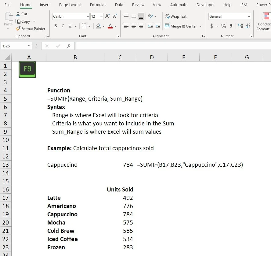
To find out the total cappuccinos sold, you’d click on an empty cell and type =SUMIF(B17:B23,”Cappuccino”,C17:C23). Here’s what’s happening with this conditional sum:
B17:B23is the range where Excel will look for the criteria."Cappuccino"is the criteria – Excel will look for this exact text.C17:C23is the sum range – Excel will add up the corresponding values from these cell references.
Press Enter, and boom! Excel gives you the total number of cappuccinos sold. No manual counting, no mistakes, just the info you need, right when you need it.
SUMIFS
Now, let’s say you’re not just interested in your coffee expenses, but you want to know how much you’ve spent on lattes specifically, and only during weekdays. Enter SUMIFS, the supercharged version of SUMIF. It allows you to add up numbers based on multiple conditions. It’s like having your cake and eating it too, only with less guilt and more data.
How To Use SUMIFS
Let’s get back to our beloved coffee shop. Your business is booming and you’ve expanded your tracking spreadsheet. Now, in addition to drink type (Column A) and units sold (Column B), you’re also keeping track of the day of the week each sale was made (Column C).
It’s Sunday evening, and as you’re enjoying your well-deserved “me” time (perhaps with a cozy latte?), you start wondering: “How many cappuccinos did I sell on Mondays last month?”
Well, Excel’s got your back! With the SUMIFS function, you can add up values based on multiple criteria. It’s like having a super-powered coffee bean counter at your fingertips!
So, here’s what you’d do: in an empty cell, type =SUMIFS(D17:D44, B17:B44, "CAPPUCCINO", C17:C44, "Monday"). Let’s break it down:
D17:D44is the sum range – these are the values that Excel will add up.B17:B44and"Cappuccino"make up our first criteria pair – Excel will only consider rows where the drink type is “Cappuccino”.C17:C44and"Monday"make up our second criteria pair – among those rows, Excel will only sum the ones where the day is “Monday”.
Hit Enter, and voila! You now know how many cappuccinos you sold on Mondays. No need to dig through piles of receipts or squint at tiny text – Excel’s got it all sorted for you!

SUMPRODUCT
Last but not least, we have SUMPRODUCT, the Hulk of the SUM family. It’s a bit more complex than its siblings, but its power is undeniable. SUMPRODUCT multiplies arrays of numbers together and then adds them up. So if you’ve ever wondered how many total calories you’ve consumed from those weekday lattes (again, maybe it’s better not to know), SUMPRODUCT has your back.
How To Use SUMPRODUCT
Let’s head back to our beloved coffee shop, where the aroma of freshly ground beans meets the clatter of tapping keys. We’ve been tracking not only the type of drinks we sell (Column A) and the quantity sold (Column B), but also their individual prices (Column C).
Now, imagine it’s the end of a particularly busy day. The last customer has left, the chairs are up, and you’re wondering: “How much revenue did I make from cappuccinos today?” Sure, you could whip out your calculator and start multiplying and adding, but why do that when Excel can serve up the answer, piping hot and error-free?
Enter the SUMPRODUCT function. It’s like having a barista that brews your coffee and tallies up your sales! Here’s how it works:
In an empty cell, type =SUMPRODUCT(C17:C44,D17:D44). This might look like a recipe for some exotic coffee blend, but let me break it down:
(C17:C44)represents the quantity of each drink sold.(D17:D44)represents the price of each drink.
What SUMPRODUCT does is multiply the quantity by the price for each item sold, and then add up these totals to give you your total revenue. It’s like having your cake and eating it too, or in this case, selling your coffee and counting it!

Pro Tips and Tricks
Next, I’ve got some secret sauce to share with you – pro tips and tricks that can take your SUM game from ‘just getting by’ to ‘Excel-lent’.
1. AutoSum Magic: Did you know there’s a magic button that can do the summing for you? Click on the cell where you want your total to appear, then click the ‘AutoSum’ button (it looks like a Greek ‘E’) on the ‘Home’ or ‘Formulas’ tab. Excel will guess the range you want to add, and often it gets it right. If not, just select the correct range, hit enter, and voila! Instant sum.
2. Quick Addition with Alt + = : Here’s a keyboard shortcut to make you feel like an Excel wizard. Select the cells you want to add up, then press Alt + =. Excel will automatically insert the SUM formula. It’s like having a mini calculator at your fingertips.
3. SUMIF/SUMIFS with Wildcards: When using SUMIF or SUMIFS, you can use wildcards in your criteria. The asterisk () represents multiple characters, and the question mark (?) represents a single character. For example, if you want to sum all sales for products starting with ‘A’, you can use “A” as your criteria. It’s like playing a game of hide-and-seek with your data, and you’re always the winner.
4. Don’t Forget Negative Numbers: Remember, the SUM function adds all numbers, including negative ones. So if you’re wondering why your sum is lower than expected, check for any pesky negative numbers throwing off your total.
Remember, mastering Excel is like learning to play an instrument. You start off with the basics, but with practice, you can create beautiful, harmonious ‘data music’. And just like any skilled musician, you’ll develop your own style and tricks along the way.
Common Mistakes and How to Avoid Them
My fellow Excel explorers, we’ve had a lot of fun on our SUM function adventure. But now, let’s take a moment to talk about something a little less fun, but just as important: mistakes.
Before we get into it, I want you to remember something. Everyone – and I mean everyone, even seasoned Excel veterans – makes mistakes. It’s all part of the learning process. So, don’t sweat it if you’ve made one, two, or even a dozen errors while practicing your SUM functions. In fact, give yourself a pat on the back. Why? Because every mistake is an opportunity to learn and grow.
So, without further ado, let’s review some of the most common SUM function pitfalls and how to sidestep them like a pro.
1. Incorrect Range Selection: This is by far the most common error. You might accidentally select an extra cell, or miss some cell references. It’s easy to do, especially when dealing with large datasets. The fix? Double-check your range before hitting enter. Taking a few extra seconds to review can save you a heap of trouble down the line.
2. Forgetting the Equals Sign: Every Excel function starts with an equals sign (=). If you forget it, Excel won’t recognize your formula and will treat it as text. Always start your formulas with = and you’ll be golden.
3. Not Accounting for Empty Cells Or Text: If there are empty cells in your range, Excel will treat them as zeros. This might not affect your SUM result, but if you’re averaging or multiplying, it could throw off your calculations. A good rule of thumb is always to fill in your data completely. Also remember that SUM functions can only use numeric values and will ignore text values.
4. Case Sensitivity in SUMIF/SUMIFS: Here’s a gotcha that trips up many folks. SUMIF and SUMIFS aren’t case-sensitive. So if you’re trying to sum data based on text criteria, remember that ‘APPLES’, ‘apples’, and ‘Apples’ will all be treated the same.
5. Overcomplicating Formulas: Sometimes, we get so caught up in using fancy functions that we forget the basics. Always ask yourself: is there a simpler way to do this? Often, a basic SUM will do the job as well as a more complicated function.
Quick Recap
We started off with the basics, getting cozy with the standard SUM function – the bread and butter of Excel. Then, we dove headfirst into the deep end, exploring the power of SUMIF, SUMIFS, and SUMPRODUCT. We played detective with our data, added conditions, and multiplied arrays like pros. We even navigated wildcards and negative numbers!
Along the way, we laughed, we learned, and yes, we made a few mistakes. But remember, it’s not about being perfect; it’s about growing and learning. And in that spirit, I’m incredibly proud of how far we’ve come.
But don’t stop now! Consider this the beginning of your Excel adventure. A whole universe of functions, formulas, and features is waiting for you to explore. So keep practicing, keep experimenting, and most importantly, keep having fun with it.
I’d love to hear about your experiences, your victories, your challenges, and your questions. After all, we’re all in this together. So, drop a comment, send an email, or share a post. Let’s turn this from a monologue into a dialogue, and create a community of Excel enthusiasts who support and learn from each other.
Frequently Asked Questions
How do I sum different cells in Excel?
To sum different cells in Excel, use the SUM function and separate each cell reference with a comma. For instance, =SUM(A1, C1, E1) will add the values in cells A1, C1, and E1.
What is the formula for the sum of a column in Excel?
The formula to sum an entire column in Excel is =SUM(column:column). For example, =SUM(A:A) will sum all the numbers in column A.
What are the 3 ways we can do a SUM function in an Excel?
The three ways to perform a SUM function in Excel are:
- Using the SUM function manually (e.g.,
=SUM(A1:A5)). - Using the AutoSum feature on the Home or Formulas tab.
- Using the keyboard shortcut Alt + = after selecting the desired cells.
How do I SUM just visible cells?
Sometimes, when you manually hide rows or use AutoFilter to display only certain data, you only want to sum the visible cells. You can use the SUBTOTAL function. If you use a total row in an Excel table, any function you select from the Total drop-down will automatically be entered as a SUBTOTAL function. You can manually type =SUBTOTAL(9, range) to sum only visible cells in a specific range.
How do I SUM multiple rows in Excel?
To sum multiple rows in Excel, use the SUM function and specify the range that covers the rows. For example, =SUM(A1:A10) will sum the values from row 1 to row 10 in column A.
How do you SUM above cells in Excel?
To sum above cells in Excel, select the cell where you want the total to appear. Then, use the SUM function and specify the range of cells above. For instance, if you want to sum A1 through A3 in cell A4, you’d write =SUM(A1:A3) in cell A4.
What is AutoSum?
AutoSum is a powerful feature in Excel that automatically enters the SUM function into a cell. It’s found on the Home or Formulas tab and looks like a Greek ‘E’. When you click it, Excel guesses the range you want to sum based on the location of your selected cell.
How do I sum only numbers in Excel?
The SUM function in Excel will automatically only sum numeric values. If your range includes text values, the calculation will ignore those cells.
How do I sum a column in an Excel table?
To sum a column in a table, you would use the SUM function and specify the range within the Excel table. For example, =SUM(Table1[Column1]) would sum all the numbers in Column1 of Table1.
How do you SUM text values in an Excel formula?
Excel cannot perform mathematical operations on text values. However, if you want to join or “sum” text from different cells, you can use the ampersand (&) or the CONCATENATE function. For example, =A1&B1 or =CONCATENATE(A1, B1) will join the text in cells A1 and B1.
Have any questions Are there other topics you would like us to cover? Leave a comment below and let us know! And make sure to subscribe to our Newsletter to receive exclusive financial news right to your inbox.