
Master The Excel Index Function Step-By-Step
Are you ready to transform your Excel skills from ‘just getting by’ to ‘absolute wizardry’?
If so, I’ve got a secret weapon that will make you the Gandalf of spreadsheets: the Index Function. This little-known tool is like having a GPS for your data – it navigates through the wilderness of numbers and takes you straight to the information you need.
Picture this: It’s late on a Friday afternoon. You’re stuck at your desk, scrolling through an Everest-sized spreadsheet, trying to find one elusive piece of data. We’ve all been there, haven’t we? I certainly have. Then, like a knight in shining armor, a colleague introduced me to the Index Function. And just like that, my Excel life was forever changed.
So, buckle up, data enthusiasts! We’re about to embark on a journey that will turn you into an Excel maestro. Let’s dive into the magical world of the Index Function together. Trust me; it’s going to be a game-changer!
Quick Overview
The INDEX function in Excel is like your personal data detective. It helps you retrieve specific data from a range or array based on its position. Imagine you’ve got a long list of names, and you want to find the 10th name on the list. Instead of counting down each row, you can use the INDEX function to instantly fetch that information.
To use the INDEX formula, you write =INDEX(array, row_num, [column_num]) into a cell, replacing ‘array’, ‘row_num’, and ‘[column_num]’ with your specific values.
Understanding the Index Function In Excel
Alright, folks! It’s time to roll up our sleeves and get down to business. Let’s talk about the Index Function.
The Index Function in Excel is a bit like your favorite GPS system. You tell it where you want to go (the data you’re looking for), and it shows you the quickest route to get there (points you directly to the cell where the data resides).
In technical terms, the Index Function returns a value or the reference to a value from within a table or range. There are two ways to use this function:
- If you want to retrieve a specific value, you use the ‘array’ format.
- If you want a reference to the specified cell, you use the ‘reference’ format.
Think of it like ordering a pizza. The ‘array’ format is like telling the pizza place, “I want the large pepperoni pizza.” You know what you want, and you ask for it directly. The ‘reference’ format, on the other hand, is like saying, “I want the pizza that’s third on your menu.” You don’t know exactly what it is, but you know where to find it.
Now, let’s not sugarcoat it – Excel can sometimes feel like trying to solve a Rubik’s cube blindfolded. We’ve all had those moments where we stare at the screen, wondering if we wouldn’t be better off crunching numbers with an abacus. But fear not, my friends! We can tame the Excel beast with tools like the Index Function and make it work for us.
What The Excel Index Function Can Do
Say goodbye to the endless scrolling and the Ctrl + F function that often feels like playing “Where’s Waldo?” with your data. The Index Function is here to save the day!

Here are its top five capabilities that make it a game-changer for managing your business finances:
- The Guidance Counsellor of Data: Just like a guidance counselor helps you find the right path in school, the Index Function guides you straight to the data you need. No more aimless wandering through rows and columns. It’s like having your own personal Excel GPS!
- The Time-Saver: Remember those days when you’d spend hours hunting for a specific piece of data? Well, with the Index Function, those days are as gone as floppy disks. It’s all about efficiency now, my friends!
- The Flexible Friend: The beauty of the Index Function is its flexibility. It covers you whether you’re looking for a specific value (‘array’ format) or a cell reference (‘reference’ format). It’s like a Swiss Army knife for your spreadsheet!
- The Complexity Tamer: Financial data can be as tangled as a box of old Christmas lights. But the Index Function cuts through the complexity, making it as easy to manage as sorting your socks.
- The Multitasker: The Index Function isn’t just a one-trick pony. Combine it with other functions like MATCH, and you’ve got yourself a dynamic duo that can tackle even the most complex financial tasks. It’s like Batman and Robin for your spreadsheet!
So, there you have it. The Index Function: your guiding light in the dark forest of financial data. It’s not just a tool; it’s a superhero waiting to save your day!
Let me share a real-life example. Imagine you’re working on a year-end report, and you need to find the total sales for a specific product in the third quarter. Your spreadsheet is a sprawling metropolis of numbers spreading across hundreds of rows and columns. You could manually hunt down this information or use the Index Function. With a few clicks, it’ll take you right to the cell you need. It’s like having a VIP pass to your data!
Or consider this: You’re forecasting next year’s budget and need the expense data from two years ago. Again, the Index Function comes to your rescue, locating the exact cell with the precision of a homing pigeon.
Step-by-Step Guide to Using the Index Function
Alright, folks! Grab your coffee, adjust your glasses, and let’s get down to the nitty-gritty of using the Index Function. Don’t worry; it’s like learning to ride a bike – a bit tricky at first, but once you’ve got it, you’ll be cruising through your spreadsheets quickly!
Step 1: Setting up your Excel sheet
Think of your Excel sheet as your workspace. You wouldn’t bake a cake without prepping your kitchen, right? So, let’s start by organizing our data. Make sure your rows and columns are labeled clearly. Remember, a tidy spreadsheet is a happy spreadsheet!
Step 2: Writing your first Excel Index Function
Now we’re ready for the fun part – writing your first Index Function! It’s like casting a magic spell, only your wand is your keyboard.
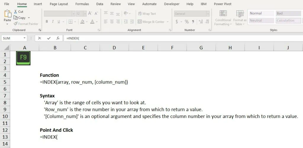
Here’s the formula: =INDEX(array, row_num, [column_num]).
- ‘Array’ is the range of cells you want to look at.
- ‘Row_num’ is the row number in your array from which to return a value.
- ‘[Column_num]’ is an optional argument and specifies the column number in your array from which to return a value.
There are two ways to write the Index Function:
The ‘Point and Click’ Method
- Start by typing the ‘=INDEX(‘ formula into the cell where you want your result to appear. It’s like saying “Open Sesame” to the Excel genie.
- Now, click and drag the mouse over the range of cells that make up your array. This is your data playground where Excel will hunt for your value.
- Type a comma, then enter the row number, another comma, and finally the column number. Remember, Excel likes its instructions clear and concise, like a coffee order at your favorite café.
- Close the bracket, hit enter, and voila! The excel index function returns your value as if by magic.
The Formula Builder Method
Remember when we were kids and we had those fabulous Lego sets? You know, the ones where you could build magnificent castles, space stations, or even entire cityscapes. Well, guess what? Excel has its own version of Legos, and it’s called the Formula Builder! So, buckle up because today, we’re going to channel our inner child and build an Index function, brick by brick.
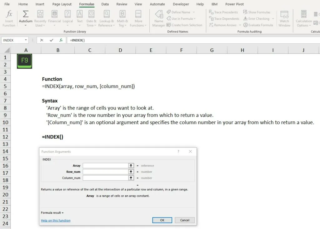
- First things first, let’s open our toolbox. Click on the cell where you want your answer to appear. Then head up to the toolbar, find the ‘fx’ symbol (it’s like the bat signal for formulas!) and click on it. This will open up the Formula Builder, your personal Excel playground.
- Now, in the box that says ‘Search for a function’, type in ‘INDEX’. It’s like asking the Lego box for a specific brick. Click on ‘INDEX’ in the list and then hit ‘OK’.
- You’ll now see a new box that says ‘Function Arguments’. This is where the real magic happens. It’s like the instruction manual for your Lego set.
- In the ‘Array’ field, enter the range of cells where your data lives. Just as you’d pick your Lego base, this is where your function will be built upon.
- The ‘Row_num’ is like choosing where to place your Lego brick on the base. Enter the row number from which you want to pull data.
- The ‘Column_num’ is optional. It’s like choosing the color of your brick. If you want data from a specific column, enter the column number here. If not, leave it blank.
Once you’ve filled in your arguments, click ‘OK’. And just like that, you’ve built your function! Your result will appear in the cell, shining like the top piece of your Lego masterpiece.
Step 3: Understanding the results and troubleshooting common errors
Congratulations! You’ve performed your first Index Function. But what if the result isn’t what you expected?
No need to panic. Let’s roll up our sleeves and tackle some of the most common errors when using the Index Function, and how to solve them.
1. #REF! Error
If Excel were a dog, the #REF! error would be its bark. It’s basically Excel’s way of saying, “Hey, I can’t find the reference you’re pointing me to!” This often happens when the row or column number provided is larger than the array dimensions.
How to Solve: Double-check your array range and make sure the row and column numbers you’re specifying actually exist within that range. It’s like making sure you’re not trying to order a latte at a burger joint!
2. #VALUE! Error
Ah, the #VALUE! error. This is like Excel’s polite way of saying, “I’m sorry, but what you’re asking doesn’t make any sense.” This often happens when the row or column number isn’t a number at all, or isn’t provided when it should be.
How to Solve: Make sure you’re providing numerical values for the row and column numbers. And remember, if you’re only specifying the row number, make sure your array is a single row or column. It’s like ensuring you’re putting the right key in the right lock!
3. #N/A Error
This one’s a classic. The #N/A error is Excel’s version of a shrugged shoulder. It’s saying, “I looked, but I couldn’t find what you’re asking for.” This can happen when you’re using the Index Function with Match, and Match can’t find the lookup value.
How to Solve: Double-check your lookup value and make sure it exists in the lookup array. If it’s there, ensure that your match type in the Match function is set correctly. It’s like making sure you’re searching for Waldo on the right page of the book!
Step 4: Advanced tips for using the Index Function
Once you’ve mastered the basics, it’s time to level up. Remember, the Index Function is even more powerful when combined with other functions. It’s like adding a turbo boost to your data analysis! For instance, pair the index and match functions to search for a specific value in an array. The possibilities are endless!
Examples and Exercises
Alright, my fellow number-crunchers, now that we’re all aboard the Index Function Express, let’s put our newfound knowledge to the test with some practical examples and a hands-on exercise. Remember, practice makes perfect – or, in our case, practice makes pristine spreadsheets!
Make sure to download our Excel workbook to follow along:
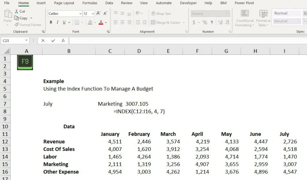
Example 1: Using the Excel Index Function to manage a budget
Let’s say you’re managing a budget for your small business. You have a spreadsheet with months in the columns and expense categories in the rows. You want to find out how much you spent on marketing in July. Normally, you’d be scrolling and scanning like a hawk, but not anymore! With the Index Function, it’s as easy as Sunday morning. Just point it to your range (the expense category), specify the row position (Marketing), and the column position (July). Voila! You’ve got your answer faster than you can say “budget surplus”!
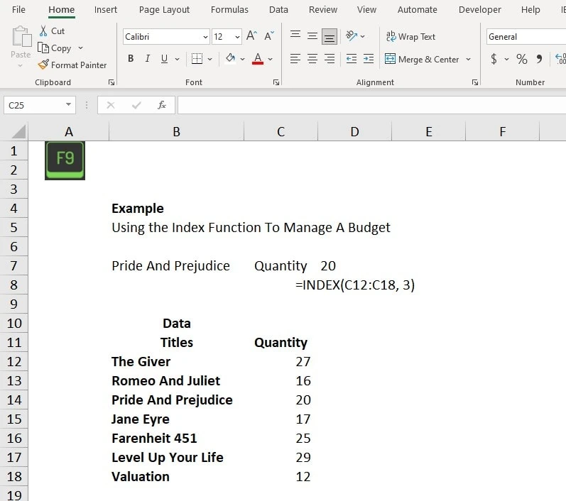
Example 2: Using the Index Function for inventory tracking
Now, imagine you’re running a bookstore (who doesn’t love the smell of new books, am I right?). You have an inventory list with book titles in one column and quantities in another. You need to know how many copies of “Pride and Prejudice” you have in stock. Instead of playing hide-and-seek with your data, you whip out the Index Function. Point it to your range (book titles), specify the row (“Pride and Prejudice”), and there you have it! Now, you can get back to recommending the perfect novel to your customers.
Exercise: Practice Using The Index Function
Your turn, friends! Let’s pretend you’re managing a team and have a list of employee names in one column and their roles in another. Use the Index Function to determine what role “Jane Doe” has in your team.
Quick Recap
Well, my friends, we’ve come to the end of our thrilling journey through the land of the Index Function. But remember, every ending is just a new beginning. This isn’t the end of your Excel mastery; it’s just the start!
You’ve bravely tackled setting up your Excel sheet, writing your first Index Function, understanding results, troubleshooting, and even some advanced tricks. Just like when I first learned to bake bread (which took more tries than I’d care to admit), the process can seem daunting. But look at you now! You’re kneading that dough of data confidently, ready to bake up a fresh financial insight.
The Index Function is more than just a formula; it’s your secret weapon in the world of business finance. It’s like having an expert navigator on your team, always ready to guide you straight to the data you need. So whether you’re managing budgets or tracking inventory, remember that the Index Function has your back.
Now, it’s your turn to join the conversation. We’re all on this journey together, learning from each other’s experiences and insights. So please don’t be shy; share your stories, successes, questions, and even your epic fails (we’ve all been there). Because in this community, every question is a chance to learn, and every mistake is just a stepping stone on the path to mastery.
Frequently Asked Questions
What is the difference between Vlookup and INDEX match?
While both Vlookup and INDEX MATCH are used to extract data, they work in different ways. Vlookup is like a loyal bloodhound, it follows a scent (or value) down a column and retrieves corresponding data from the specified column. However, it only looks rightwards. On the other hand, INDEX MATCH is more versatile. It’s like a skilled falcon, soaring above your spreadsheet, capable of looking both right and left to find the data you need.
What Is The Difference Between Index And Index Match
While they sound similar, Index and Index Match have distinct functions. Index is used to retrieve data from a table based on row and column numbers. On the other hand, the Index Match function returns data based on specific criteria, making it more flexible and powerful.
How do you INDEX match with multiple criteria?
When you want to use multiple criteria, you can combine INDEX with MATCH and use an array formula. It’s like conducting a thorough search with multiple search parameters. You’ll use MATCH to find the row and column numbers based on your criteria, and then feed those into the INDEX function to retrieve your desired value.
What is an example of an INDEX function?
Let’s say you’re managing a list of employees with their roles in a column. You could use the INDEX function to find out what role “Jane Doe” has in your team. It’s like asking Excel, “Hey, could you please tell me what role Jane Doe has?” And voila, Excel delivers!
Is INDEX function better than VLOOKUP?
While both functions have their advantages, the INDEX function (especially when combined with MATCH) offers more flexibility than VLOOKUP. It can look both right and left, and doesn’t require your lookup value to be in the first column of your range. So, it’s like having a four-wheel drive for your data journey, capable of navigating even the trickiest terrains of your spreadsheet.
Have any questions? Are there other topics you would like us to cover? Leave a comment below and let us know! Make sure to subscribe to our Newsletter to receive exclusive financial news right to your inbox.